AmoebotSim 2.0
As part of our research on programmable matter, we developed the simulation environment AmoebotSim 2.0 for the geometric amoebot model, focusing on the reconfigurable circuit and joint movement extensions of the model. The source code and documentation pages are available on GitHub.
AmoebotSim 2.0 was inspired by AmoebotSim, a simulator for the geometric amoebot model without extensions, which is currently maintained by members of the Self-Organizing Particle Systems (SOPS) Lab. While AmoebotSim supports the geometric amoebot model with a sequential scheduler (exactly one amoebot is active in each time step), the model extensions supported by AmoebotSim 2.0 require a fully synchronous scheduler (all amoebots are active simultaneously in each time step).
Below, we showcase the most important features of the simulator, followed by several example algorithms. For installation instructions, user guides and technical documentation, please refer to the documentation. You can also run the simulator in the browser using our web build:
Movement and Beep Animations
Movement Animations
The joint movement extension allows amoebots to push and pull each other during their movements. In just a single round, the positions of the amoebots in the structure can change drastically. Smooth animations with variable speed make even the most complex joint movements comprehensible. They can also help identifying potential for collisions when moving parts of the structure get very close to each other, even if no collision occurs yet.
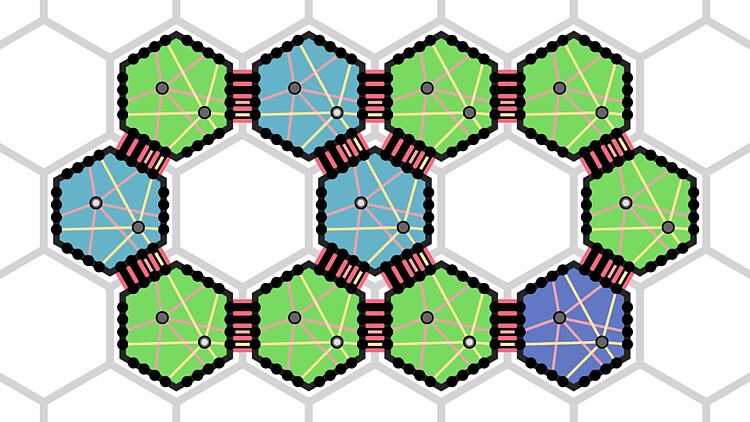
Beep Animations
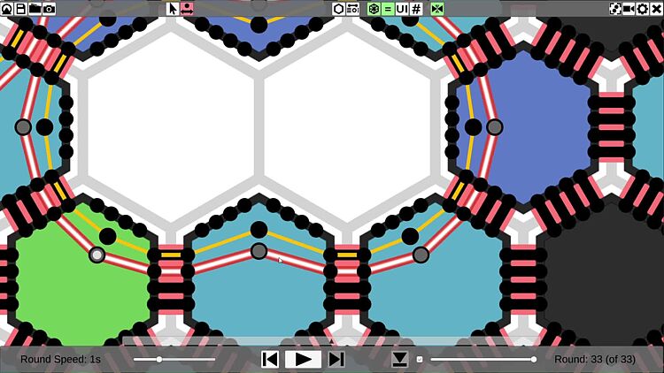
With the reconfigurable circuit extension, amoebots can construct circuits and use them as simple communication networks. The simulator places flashing highlights on circuits where beeps were sent to make them stand out from other circuits more. Additionally, partition sets (the black circles inside the amoebots) have a gray highlight when they receive a beep and a white center when they send a beep.
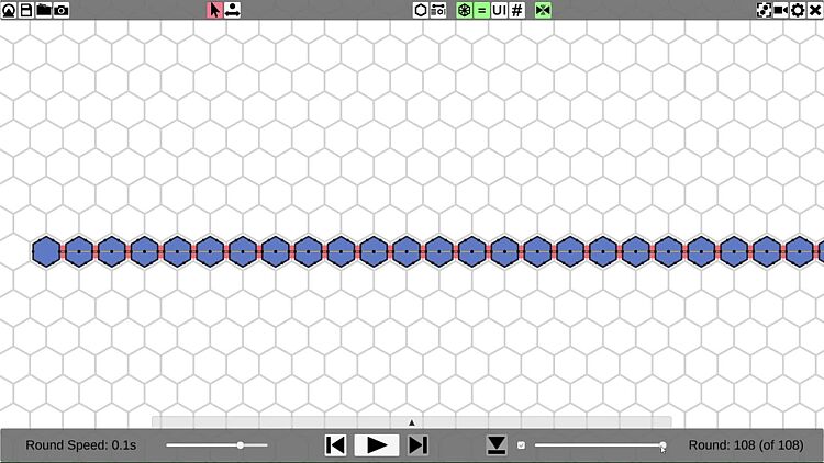
Flexible Simulation History
The simulator records all rounds of an algorithm execution. Using a slider or buttons, you can rewind to any round of the simulation to inspect and replay previous system states. You can also cut off the history after the selected round and run the simulation again from the current round. If the algorithm is randomized or you edited the states of some amoebots, the simulation may show a different behavior.
Customizable Appearance
The visual representation of the amoebot structure can be customized in various ways. In the program code, you can set the colors of amoebots and circuits, and place the partition sets inside the amoebots arbitrarily. In the UI, you can switch between hexagon, circle and graph view modes. To declutter the viewport, you can toggle the display of circuits and bonds. The UI can be hidden for better visibility or to make recordings, and the camera can be rotated in 30° steps. The partition set move tool allows you to temporarily move partition sets with the cursor to make a pin configuration more readable.
UI Features


Example Algorithms
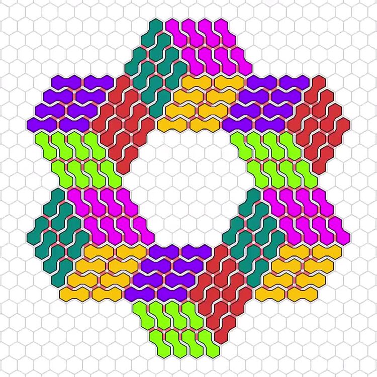
Inner and Outer Boundary Test
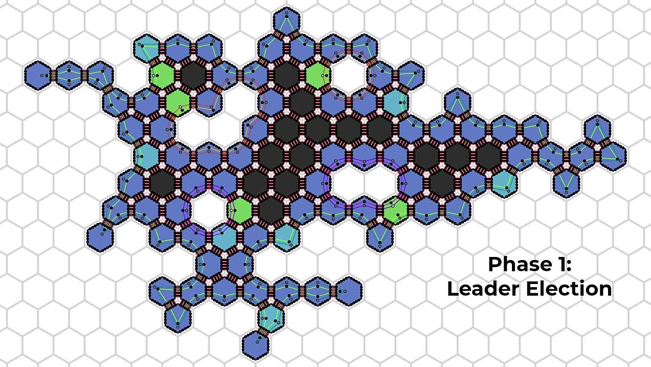
A boundary is a set of amoebots that are adjacent to the same unoccupied component of the triangular grid. There is always a unique outer boundary that is adjacent to the infinite unnocupied component of the grid graph. Every other boundary belongs to a hole in the structure. In the inner and outer boundary test algorithm, the amoebots use circuits to determine which of the boundaries is the outer boundary. As a byproduct, they also elect a leader on every boundary. Note that an amoebot may belong to up to three distinct boundaries. The algorithm we describe here was introduced by Derakhshandeh et al. and accelerated with circuits by Padalkin et al.
The algorithm starts with a leader election procedure which is based on random coin tosses. The amoebots on each boundary run a competition where in each round, every remaining candidate tosses a coin. The coin toss results are sent on a circuit connecting the boundary, letting all amoebots know which results occurred. If both Heads and Tails occurred, all candidates with Tails withdraw their candidacy. Otherwise, the procedure stops. To boost the probability that only one candidate remains, a new and independent competition with auxiliary candidates is started. During each step, the original candidates perform another round of their competition. By restarting the auxiliary competition several times, the success probability can be increased even further. Additionally, the competition on each boundary is continued until all boundaries have finished their respective leader election. The synchronization between the boundaries is accomplished by a global circuit that spans the entire amoebot structure.
In the second phase, each boundary computes the sum of turn angles that accumulates during one traversal of the boundary. For the outer boundary, the sum is 360°, and for every inner boundary, it is -360°. Because only turns by multiples of 60° are possible in the triangular grid and because intermediate sums can get arbitrarily large, the amoebots sum the number of 60° turns modulo 5 instead. The resulting sum for the outer boundary is 6 mod 5 = 1 and the sum for an inner boundary is -6 mod 5 = 4. Using circuits, the amoebots compute this sum in a parallelized fashion, similar to an adder tree. In each step, half of the remaining partial sums are added to the other half. As a result, the number of steps is only logarithmic in the length of the boundary.
Line Formation
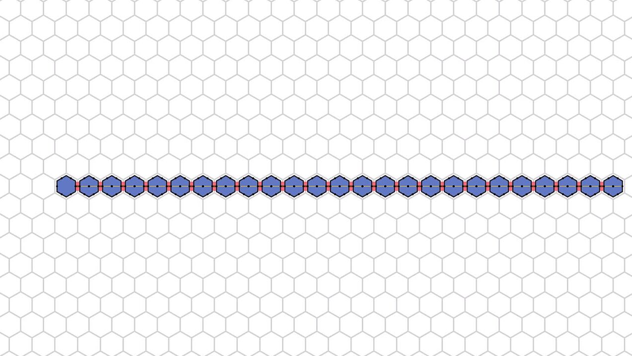
In the line formation algorithm, a single amoebot has been elected as the leader and chooses a direction in which to build a line. The other amoebots then have to move so that the structure eventually forms a straight line extending from the leader in the chosen direction. This algorithm does not use joint movements and is not improved by circuits, but it showcases the movement animations and some UI features of the simulator. It was first presented by Derakhshandeh et al.
The amoebots can be categorized into four classes: Amoebots that have already reached their position on the line (yellow), amoebots that are adjacent to the line and therefore know where to move (red), amoebots that are not adjacent to the line but already know where to move (blue), and amoebots that do not know where to move yet (black). By checking the state of its neighbors, an amoebot can update its role. For example, a contracted amoebot finding itself in front of an amoebot that is part of the line knows that it has reached its own position on the line. Amoebots that are not adjacent to the line but have a neighbor that knows where to move (red or blue) remember this neighbor as a parent and follow their parent until they reach the line. This creates a tree structure (visualized by the blue arrows) that eventually reaches all amoebots. Since no amoebot ever moves along the line towards the leader, the completed part of the line is recognized by amoebots without any neighbors outside of the line. These amoebots construct a circuit that connects the completed part of the line. When the last amoebot realizes that it is part of the completed line, it beeps on the circuit to inform all amoebots about the completion.
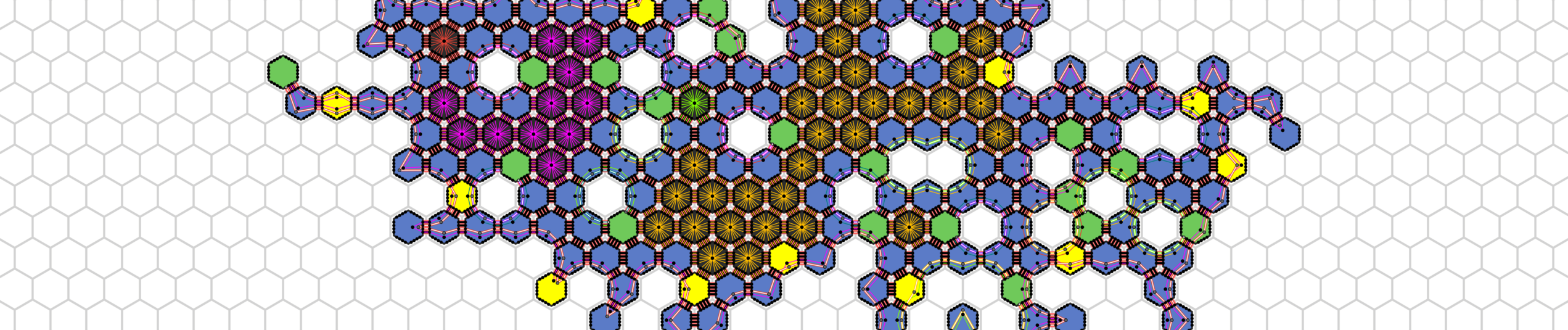
Shortest Path Tree Construction
In the single-source shortest path problem, a single amoebot is marked as a source and some other amoebots are marked as destinations. The amoebots must compute shortest paths connecting the source to all destinations. To accomplish this, they use axis-aligned portals, which are visualized on top of the amoebot structure in the simulator. This algorithm was presented by Padalkin and Scheideler. It only works for amoebot structures without holes.
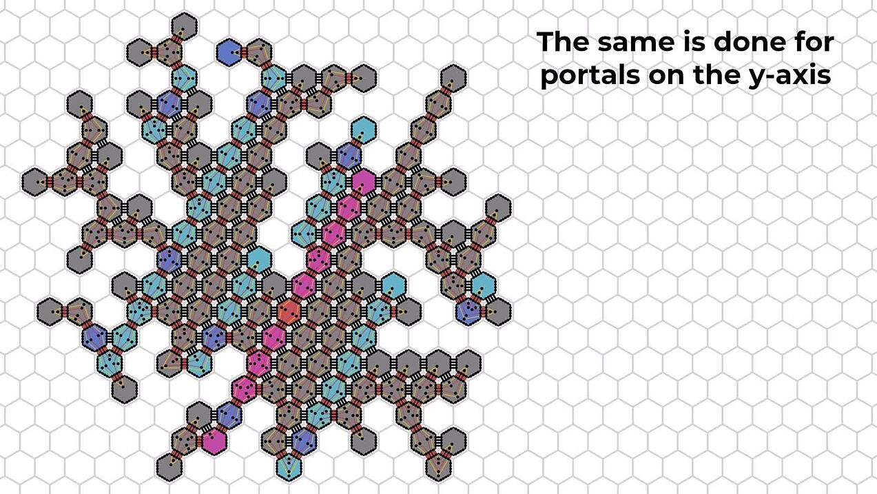
An x-portal is a maximal connected set of amoebots on the same line parallel to the x- (horizontal) axis. Portals for the y- and z-axes are defined similarly. The amoebots can easily establish these portals and identify the "leftmost" edge between two adjacent portals as the unique edge connecting the portals. Because the amoebot structure has no holes, the resulting graph with portals as nodes is a tree. If we mark the portal containing the source amoebot as the root, every portal has a unique parent portal, and every amoebot in turn has at most two neighbors belonging to the parent of its own portal.
It can be shown that for any amoebot u, a neighbor v lies on a shortest path from u to the source if and only if v belongs to the parent portal of u for the portal trees of two axes. Therefore, the algorithm constructs the portal trees for all three axes, allowing each amoebot to identify its parent portals. This is done by constructing circuits along an in-order traversal of the portal tree and counting the number of destinations encountered along this traversal. The traversal visits every edge in the portal tree twice, once moving away from the root and once moving back toward the root. If the subtree of an edge contains a destination, the number of destinations counted before the first visit is lower than the number of destinations encountered before the second visit. By comparing these numbers, the amoebots determine the directions of all edges in the portal tree.
Each amoebot counts how many times each neighbor occurred as a portal parent. If any neighbor occurred twice, the amoebot chooses such a neighbor as its parent in the shortest path tree. For some amoebots, such a neighbor does not exist. These amoebots can immediately prune themselves from the tree. After this step, there can still be subtrees that do not contain any destinations and some parts of the amoebot structure may not be connected to the shortest path tree by parent edges. To prune these superfluous amoebots, a traversal of the current shortest path tree is used to construct circuits and count occurrences of destinations like before. Disconnected parts will not receive any beeps at all and subtrees without destinations will have equal destination counts on all edges. After pruning these amoebots, only shortest paths from the destinations to the source remain.
Citation
If you use AmoebotSim 2.0 for your research, please cite the project as follows:
Matthias Artmann, Tobias Maurer, Andreas Padalkin, Daniel Warner. "AmoebotSim 2.0: A Visual Simulation Environment for the Amoebot Model with Reconfigurable Circuits and Joint Movements", available online at https://github.com/martmannupb/AmoebotSim-2.0, 2025.
Contact
> Theory of Distributed Systems
Research Associate
Office: F2.323
Phone: +49 5251 60-6704
E-mail: matthias.artmann@uni-paderborn.de
> Theory of Distributed Systems
Research Associate
Office: F2.406
Phone: +49 5251 60-6725
E-mail: padalkin@mail.uni-paderborn.de
Office hours:
nach Vereinbarung